Conditional Probability Calculator
Complete statistics guide • Step-by-step solutions
Conditional Probability::
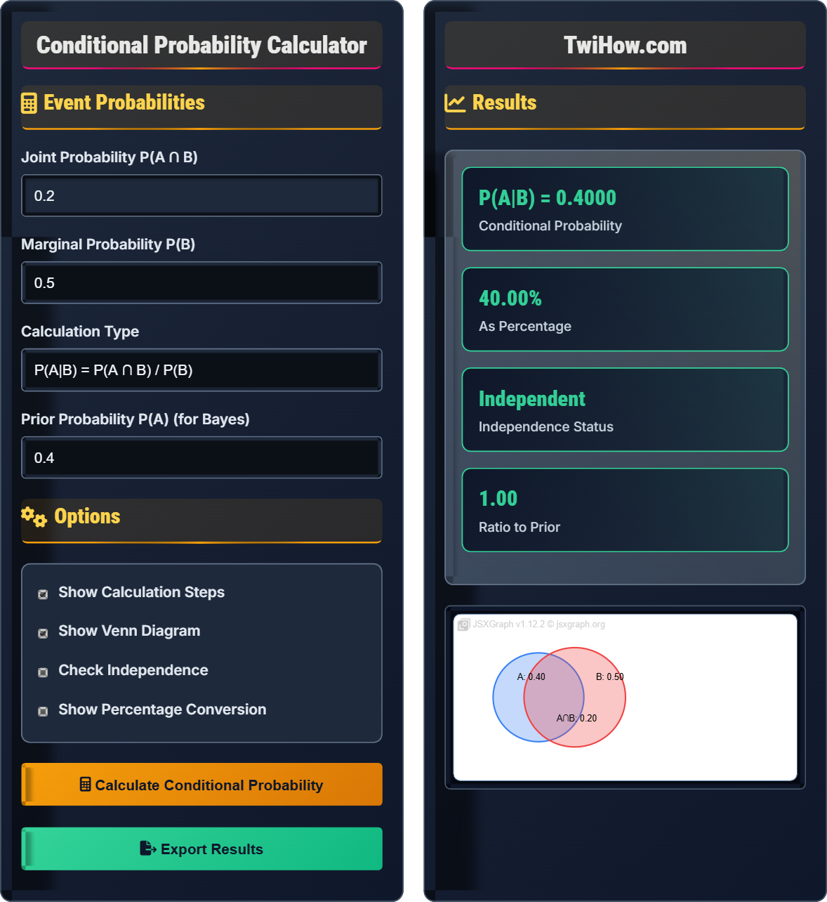
Show the calculator /Simulator\( P(A|B) = \frac{P(A \cap B)}{P(B)} \)
Conditional probability measures the likelihood of event A occurring given that event B has already occurred. It quantifies how the probability of one event changes when we have information about another related event. This fundamental concept in probability theory is essential for understanding dependent events, statistical inference, and decision-making under uncertainty.
Where:
- \(P(A|B)\) = probability of A given B
- \(P(A \cap B)\) = joint probability of A and B
- \(P(B)\) = marginal probability of B
Conditional probability is crucial in many fields including medical diagnosis, machine learning, finance, and quality control. It allows us to update our beliefs about the likelihood of events based on new information, forming the basis for Bayes' theorem and modern statistical inference.
Event Probabilities
Options
Results
| Event | Probability | Symbol | Interpretation |
|---|
Enter probabilities to see calculation steps.
Additional statistics will appear here.
Conditional Probability Explained
Conditional probability measures the likelihood of an event occurring given that another event has already occurred. It quantifies how the probability of one event changes when we have information about another related event. This concept is fundamental to understanding dependent events and forms the basis for Bayesian inference, medical diagnosis, and decision-making under uncertainty.
The fundamental conditional probability formula is:
Additionally, we have:
Where:
- \(P(A|B)\) = probability of A given B
- \(P(B|A)\) = probability of B given A
- \(P(A \cap B)\) = joint probability of A and B
- \(P(A)\) = marginal probability of A
- \(P(B)\) = marginal probability of B
Key characteristics of conditional probability:
- Range: Always between 0 and 1 (inclusive)
- Dependence: Reflects relationship between events
- Reduction: P(A|A) = 1 (certainty given itself)
- Chain Rule: P(A ∩ B) = P(A|B) × P(B)
- Medical Diagnosis: Probability of disease given symptoms
- Machine Learning: Classification and prediction
- Finance: Risk assessment given market conditions
- Quality Control: Defect probability given test results
Conditional Probability Fundamentals
Conditional probability measures the likelihood of event A occurring given that event B has already occurred.
\( P(A|B) = \frac{P(A \cap B)}{P(B)} \)
Where P(A|B) = probability of A given B.
- P(B) > 0 (conditioning event must be possible)
- 0 ≤ P(A|B) ≤ 1
- P(A|B) = 1 if A ⊆ B
- P(A|B) = 0 if A ∩ B = ∅
Applications
Foundation for Bayes' theorem, likelihood ratios, and statistical inference.
- Medical testing and diagnosis
- Spam detection in email
- Weather forecasting
- Customer behavior prediction
- Events must be properly defined
- Conditioning event must have non-zero probability
- Directionality matters (P(A|B) ≠ P(B|A))
- Context affects probability estimates
Conditional Probability Learning Quiz
In a deck of 52 cards, what is the probability of drawing a heart given that the card drawn is red?
Step 1: Define the events
A = Card is a heart
B = Card is red
Step 2: Identify relevant counts
Red cards in deck = 26 (hearts + diamonds)
Hearts in deck = 13
Red hearts = 13 (all hearts are red)
Step 3: Apply conditional probability formula
P(Heart | Red) = P(Heart ∩ Red) / P(Red) = (13/52) / (26/52) = 13/26 = 1/2
The answer is A) 1/2.
Conditional probability reduces the sample space to only those outcomes where the conditioning event occurs. Here, since we know the card is red, we only consider the 26 red cards (not all 52 cards). Of these red cards, 13 are hearts, giving us a probability of 13/26 = 1/2. This demonstrates how conditional probability updates our belief based on new information.
Conditional Probability: Probability of A given B has occurred
Sample Space Reduction: Limiting outcomes to those satisfying condition
Joint Event: Both A and B occurring simultaneously
• P(A|B) = P(A ∩ B) / P(B)
• Sample space reduced to outcomes where B occurs
• P(B) must be greater than 0
• Always identify the conditioning event
• Reduce sample space to B outcomes
• Count favorable outcomes within B
• Forgetting to reduce the sample space
• Confusing P(A|B) with P(B|A)
• Not verifying P(B) > 0
A certain disease affects 1% of the population. A test for the disease is 95% accurate (if you have the disease, there's a 95% chance of testing positive; if you don't have the disease, there's a 95% chance of testing negative). What is the probability that a person has the disease given that they tested positive?
Step 1: Define events and probabilities
D = person has disease
T = person tests positive
P(D) = 0.01 (1% prevalence)
P(D') = 0.99 (99% don't have disease)
P(T|D) = 0.95 (test accuracy if disease present)
P(T|D') = 0.05 (false positive rate)
Step 2: Calculate joint probabilities
P(T ∩ D) = P(T|D) × P(D) = 0.95 × 0.01 = 0.0095
P(T ∩ D') = P(T|D') × P(D') = 0.05 × 0.99 = 0.0495
Step 3: Calculate total probability of positive test
P(T) = P(T ∩ D) + P(T ∩ D') = 0.0095 + 0.0495 = 0.059
Step 4: Apply conditional probability formula
P(D|T) = P(T ∩ D) / P(T) = 0.0095 / 0.059 = 0.161 (approximately 16.1%)
Despite the test being 95% accurate, the probability of having the disease given a positive test is only about 16.1%. This counterintuitive result occurs because the disease is rare in the population.
This example demonstrates the importance of considering base rates (prevalence) when interpreting test results. Even with a highly accurate test, if the condition is rare, most positive results will be false positives. This is a fundamental concept in medical statistics and diagnostic testing, showing how conditional probability helps interpret screening results in real-world contexts.
Prevalence: Rate of disease in population
False Positive: Test positive when condition absent
Base Rate: Prior probability of condition
• Consider base rates when interpreting tests
• P(A|B) ≠ P(B|A) in general
• Accuracy ≠ probability of condition given test
• Always consider the base rate of condition
• Use tree diagrams for complex scenarios
• Calculate all relevant probabilities
• Confusing test accuracy with post-test probability
• Ignoring base rates
• Forgetting to calculate total probability of test
In a factory, 2% of products are defective. A quality control test correctly identifies 98% of defective products but also flags 3% of good products as defective. What is the probability that a product is actually defective given that it tested positive?
Step 1: Define events and probabilities
D = product is defective
T = product tests positive
P(D) = 0.02 (2% defective rate)
P(D') = 0.98 (98% good products)
P(T|D) = 0.98 (test detects 98% of defects)
P(T|D') = 0.03 (3% false positive rate)
Step 2: Calculate joint probabilities
P(T ∩ D) = P(T|D) × P(D) = 0.98 × 0.02 = 0.0196
P(T ∩ D') = P(T|D') × P(D') = 0.03 × 0.98 = 0.0294
Step 3: Calculate total probability of positive test
P(T) = P(T ∩ D) + P(T ∩ D') = 0.0196 + 0.0294 = 0.049
Step 4: Apply conditional probability formula
P(D|T) = P(T ∩ D) / P(T) = 0.0196 / 0.049 = 0.4 (or 40%)
The probability that a product is actually defective given that it tested positive is 40%.
This quality control example illustrates how even a test with high accuracy can result in many false positives when the condition being tested for is relatively rare. In this case, despite the test being 98% effective at detecting defects, only 40% of positive test results correspond to actual defects. This has important implications for resource allocation in quality control processes.
Quality Control: Process of ensuring product meets specifications
False Positive: Good product flagged as defective
True Positive: Defective product correctly identified
• P(defective|positive) ≠ test accuracy
• Consider both detection rate and false positive rate
• Base rate affects post-test probability
• Calculate all components of Bayes' theorem
• Consider cost implications of false positives
• Adjust testing thresholds based on costs
• Confusing test sensitivity with post-test probability
• Not accounting for false positive rate
• Forgetting to calculate total positive probability
Are the events "rolling an even number" and "rolling a number greater than 3" independent when rolling a fair six-sided die? Calculate P(Even|>3) and P(Even) to demonstrate your answer.
Step 1: Identify possible outcomes
Die faces: {1, 2, 3, 4, 5, 6}
Even numbers: {2, 4, 6}
Numbers > 3: {4, 5, 6}
Even and > 3: {4, 6}
Step 2: Calculate unconditional probability
P(Even) = 3/6 = 1/2 = 0.5
Step 3: Calculate conditional probability
P(Even|>3) = P(Even ∩ >3) / P(>3) = (2/6) / (3/6) = 2/3 ≈ 0.667
Step 4: Compare probabilities
P(Even|>3) = 2/3 ≠ P(Even) = 1/2
Since P(Even|>3) ≠ P(Even), the events are dependent. Knowing the roll is greater than 3 increases the probability of it being even from 50% to 66.7%.
Two events A and B are independent if P(A|B) = P(A), meaning knowledge of B doesn't change the probability of A. In this example, learning that the roll is greater than 3 changes the probability of it being even (from 1/2 to 2/3), proving the events are dependent. This demonstrates how conditional probability can be used to test independence between events.
Independent Events: Events where occurrence of one doesn't affect probability of other
Dependent Events: Events where occurrence of one affects probability of other
Testing Independence: Comparing P(A|B) with P(A)
• Independent: P(A|B) = P(A)
• Dependent: P(A|B) ≠ P(A)
• Independence is mutual: A independent of B implies B independent of A
• Compare conditional and marginal probabilities
• Use definition to test independence
• Consider if knowing one event affects the other
• Assuming events are independent without verification
• Not comparing conditional and marginal probabilities
• Confusing correlation with causation
Which of the following statements about conditional probability is TRUE?
Let's examine each option:
A) False - P(A|B) and P(B|A) are generally different unless P(A) = P(B)
B) False - Conditional probability is always between 0 and 1 inclusive
C) True - This is the fundamental definition of conditional probability
D) True - Division by zero is undefined, so P(A|B) is undefined when P(B) = 0
Both C and D are technically correct, but C represents the core definition. The fundamental formula for conditional probability is P(A|B) = P(A ∩ B) / P(B), provided P(B) > 0.
The answer is C) P(A|B) = P(A ∩ B) / P(B).
The conditional probability formula P(A|B) = P(A ∩ B) / P(B) is fundamental to probability theory. It shows how we update our probability assessment for event A when we know that event B has occurred. The conditioning event B becomes our new sample space, and we calculate the proportion of B that also satisfies A. This formula is the basis for all conditional probability calculations.
Conditional Probability: Probability of A given B has occurred
Joint Probability: Probability of A and B both occurringMarginal Probability: Probability of single event
• P(A|B) = P(A ∩ B) / P(B) when P(B) > 0
• 0 ≤ P(A|B) ≤ 1
• P(A|B) ≠ P(B|A) in general
• Remember the conditioning event is in denominator
• Joint probability is in numerator
• Verify P(B) > 0 before calculating
• Reversing the conditioning (confusing A|B with B|A)
• Forgetting to check P(B) > 0
• Not understanding the formula structure
FAQ
Q: What's the difference between P(A|B) and P(A ∩ B)?
A: P(A ∩ B) is the joint probability that both A and B occur, calculated with respect to the entire sample space. P(A|B) is the conditional probability of A occurring given that B has already occurred, calculated with respect to the subset where B occurs. The relationship is: P(A|B) = P(A ∩ B) / P(B). So conditional probability adjusts for the fact that we know B has occurred, effectively shrinking our sample space to just those outcomes where B happens.
Q: How is conditional probability used in machine learning?
A: Conditional probability is fundamental to many machine learning algorithms. Naive Bayes classifiers use P(class|features) to make predictions. Bayesian networks model relationships between variables using conditional probabilities. In deep learning, conditional probability appears in sequence models like language models (P(next word|previous words)). Conditional probability also underlies concepts like likelihood, posterior probability, and is essential for understanding uncertainty quantification in predictions.