Median Formula Calculator
Complete statistics guide • Step-by-step solutions
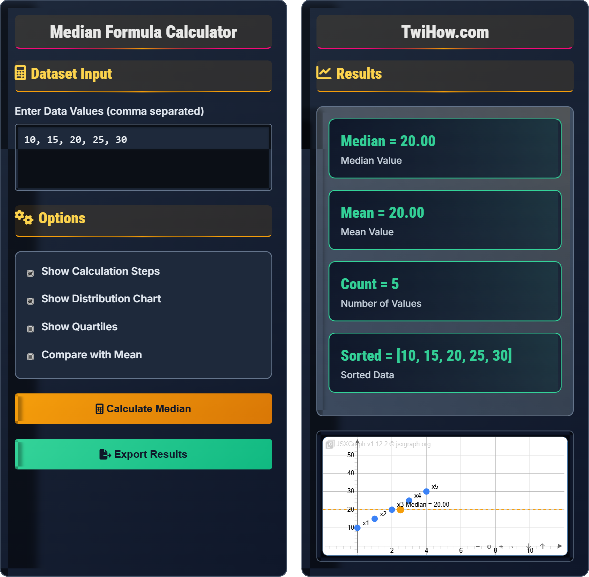
Median Formula::
Show the calculator /Simulator\( \text{Median} = \begin{cases} x_{\frac{n}{2}} & \text{if } n \text{ is odd} \\ \frac{x_{\frac{n}{2}} + x_{\frac{n}{2}+1}}{2} & \text{if } n \text{ is even} \end{cases} \)
The median is the middle value in a sorted dataset. It divides the data into two equal halves, with 50% of values below and 50% above the median. Unlike the mean, the median is robust to outliers and provides a better representation of central tendency for skewed distributions.
Where:
- \(n\) = number of values in the dataset
- \(x_i\) = values in the sorted dataset
The median is particularly useful when dealing with skewed data, ordinal data, or when outliers might distort the mean. It's a resistant measure of central tendency that maintains its position even when extreme values are present.
Dataset Input
Options
Results
| Index | Original Value | Sorted Position | Is Median? |
|---|
Enter data to see calculation steps.
Additional statistics will appear here.
Median Formula Explained
The median is the middle value in a dataset when the values are arranged in ascending or descending order. It divides the data into two equal halves, with 50% of values below and 50% above the median. The median is a robust measure of central tendency that is not affected by outliers or extreme values, making it particularly useful for skewed distributions.
The median formula depends on whether the dataset has an odd or even number of values:
Where:
- \(n\) = number of values in the dataset
- \(x_i\) = values in the sorted dataset
- \(x_{\frac{n}{2}}\) = the middle value when n is odd
- \(x_{\frac{n}{2}}\) and \(x_{\frac{n}{2}+1}\) = the two middle values when n is even
Key characteristics of the median:
- Robust to Outliers: Extreme values do not affect the median
- Position Based: Depends only on the middle position(s)
- Always Exists: Every dataset has a unique median
- Divides Data: Exactly 50% of values are below and above
- Skewed Distributions: When data is not symmetric
- Data with Outliers: When extreme values are present
- Ordinal Data: For ranked categorical data
- Income/Price Data: When distributions are typically right-skewed
Median Fundamentals
The median is the middle value of a dataset when arranged in order, dividing the data into two equal halves.
\( \text{Median} = \begin{cases} x_{\frac{n}{2}} & \text{if } n \text{ is odd} \\ \frac{x_{\frac{n}{2}} + x_{\frac{n}{2}+1}}{2} & \text{if } n \text{ is even} \end{cases} \)
Where x = sorted values, n = count.
- Data must be sorted first
- Not affected by outliers
- Exactly 50% of data on each side
- Works with ordinal data
Applications
Robust measure of central tendency, used with mean and mode.
- Income distribution analysis
- Housing price comparisons
- Performance rankings
- Medical research data
- Insensitive to data spread
- May not represent typical value
- Less mathematically tractable
- Doesn't use all data values
Median Formula Learning Quiz
What is the median of the dataset: 5, 10, 15, 20, 25?
First, sort the data: [5, 10, 15, 20, 25] (already sorted)
Count of values (n) = 5 (odd)
Median position = (n+1)/2 = (5+1)/2 = 3rd position
Median = 15 (the 3rd value)
The answer is B) 15.
The median calculation begins with sorting the data in ascending order. Once sorted, we determine the position of the middle value. For an odd number of values, the median is the value at position (n+1)/2. In this case, with 5 values, the median is at position (5+1)/2 = 3, which corresponds to the third value in the sorted list.
Median: The middle value in a sorted dataset
Sorted Order: Arranging values from least to greatest
Odd Number: A number that cannot be evenly divided by 2
• Data must always be sorted first
• For odd n: Median = value at position (n+1)/2
• For even n: Median = average of two middle values
• Always sort the data before finding the median
• Count positions carefully when n is large
• The median is always a value from the original dataset (when n is odd)
• Forgetting to sort the data first
• Counting positions incorrectly
• Using the wrong formula for odd/even n
Calculate the median of the dataset: 10, 12, 14, 16, 18, and then recalculate after adding an outlier value of 100. Compare the impact on the median versus the mean.
Original dataset: 10, 12, 14, 16, 18
Sorted: [10, 12, 14, 16, 18]
n = 5 (odd), median position = (5+1)/2 = 3
Original Median = 14
Original Mean = (10+12+14+16+18)/5 = 70/5 = 14
New dataset: 10, 12, 14, 16, 18, 100
Sorted: [10, 12, 14, 16, 18, 100]
n = 6 (even), median positions = 3rd and 4th
New Median = (14+16)/2 = 15
New Mean = (10+12+14+16+18+100)/6 = 170/6 = 28.33
The median changed from 14 to 15 (increase of 1), while the mean changed from 14 to 28.33 (increase of 14.33). The median was much less affected by the outlier.
This comparison highlights the robustness of the median compared to the mean. The median only considers the position of values, not their actual magnitudes, so an outlier at the extreme end of the distribution has minimal impact. The mean, however, incorporates the actual value of every data point, making it sensitive to extreme values. This property makes the median preferable when analyzing skewed data or data with outliers.
Robustness: Resistance to the effects of outliers
Outlier: A data point significantly different from others
Skewed Distribution: Asymmetric data distribution
• Median is robust to outliers
• Mean is sensitive to outliers
• Median uses position, mean uses magnitude
• Use median for skewed distributions
• Always visualize data to identify outliers
• Compare median and mean to assess skewness
• Assuming mean and median are always similar
• Using mean when median would be more appropriate
• Not considering the impact of outliers
A real estate agent collected the following home prices in a neighborhood: $200,000, $220,000, $230,000, $240,000, $250,000, $260,000, $1,500,000. What is the median home price? How does this compare to the mean, and which measure better represents the typical home price in this neighborhood?
Step 1: Sort the data
[$200,000, $220,000, $230,000, $240,000, $250,000, $260,000, $1,500,000]
Step 2: Find the median
n = 7 (odd), median position = (7+1)/2 = 4th position
Median = $240,000
Step 3: Calculate the mean
Mean = ($200,000 + $220,000 + $230,000 + $240,000 + $250,000 + $260,000 + $1,500,000) / 7
Mean = $3,100,000 / 7 = $442,857.14
The median ($240,000) is much lower than the mean ($442,857.14). The median better represents the typical home price because the expensive mansion ($1,500,000) significantly skews the mean upward.
This example demonstrates why the median is often preferred for real estate pricing and other economic data. The presence of one extremely expensive home inflates the mean, making it unrepresentative of typical homes in the area. The median remains stable and represents the middle value, providing a more accurate picture of what a typical home costs in the neighborhood.
Typical Value: A representative value for the dataset
Representative Measure: A statistic that reflects common values
Economic Data: Financial information used for analysis
• Median is robust to extreme values
• Mean can be skewed by outliers
• Choose measure based on data characteristics
• Always consider data distribution shape
• Look for outliers before choosing measure
• Use median for income and housing prices
• Using mean for heavily skewed data
• Not identifying outliers in economic data
• Assuming mean always represents typical value
Given the dataset: 5, 10, 15, 20, 25, 30, 35, 40, 45, 50, find the median and the first and third quartiles. Explain the relationship between these measures.
Dataset: [5, 10, 15, 20, 25, 30, 35, 40, 45, 50] (already sorted)
n = 10 (even)
Median: Positions 5 and 6 → (25 + 30) / 2 = 27.5
First Quartile (Q1): Median of lower half [5, 10, 15, 20, 25]
n_lower = 5 (odd), position = (5+1)/2 = 3 → Q1 = 15
Third Quartile (Q3): Median of upper half [30, 35, 40, 45, 50]
n_upper = 5 (odd), position = (5+1)/2 = 3 → Q3 = 40
Relationship: The median (27.5) divides the data into two equal parts. Q1 (15) marks the 25th percentile, Q2 (median) marks the 50th percentile, and Q3 (40) marks the 75th percentile. Together, they form the five-number summary along with minimum (5) and maximum (50).
Quartiles extend the concept of the median to divide data into four equal parts. Q1 is the median of the lower half, Q2 is the overall median, and Q3 is the median of the upper half. These quartiles help understand the spread and shape of the data distribution. The interquartile range (IQR = Q3 - Q1) measures the middle 50% of the data and is used to identify outliers.
Quartiles: Values that divide data into four equal parts
First Quartile (Q1): 25th percentile
Third Quartile (Q3): 75th percentile
• Q2 = Median
• Q1 = median of lower half
• Q3 = median of upper half
• Include median in both halves when n is odd
• Exclude median from both halves when n is even
• Use quartiles to identify data spread
• Including/excluding median incorrectly in halves
• Confusing quartile positions
• Not sorting data before calculating quartiles
Which of the following statements about the median is TRUE?
Let's examine each option:
A) False - Mean and median are only equal in symmetric distributions
B) False - Median is robust to outliers
C) True - By definition, the median divides data into two equal halves
D) False - Median can be calculated for any dataset size
The median specifically identifies the value that splits the dataset into two equal groups: 50% of values are below the median and 50% are above it.
The answer is C) The median divides data into two equal halves.
The defining characteristic of the median is its ability to partition data into two equal groups. This property makes it fundamentally different from other measures of central tendency. Whether the dataset has an odd or even number of values, the median always represents the point where half the data lies below and half lies above, regardless of the actual values themselves.
Equal Halves: Two groups with the same number of data points
Partition: Division of a set into separate parts
Percentile: Value below which a percentage of data falls
• Median always divides data into 50%-50% split
• Median is robust to extreme values
• Median exists for any dataset size
• Think of median as the "middle" value
• Always sort data first
• Remember 50% below, 50% above
• Confusing median with mean
• Forgetting to sort data
• Assuming median is always a value from the dataset
FAQ
Q: When should I use the median instead of the mean?
A: Use the median when your data contains outliers, is skewed, or when you want a measure that is not influenced by extreme values. The median is particularly valuable for income data, house prices, or any dataset where extreme values could distort the average. For example, in a neighborhood where most houses cost $200k but one costs $2M, the median would better represent the typical house price than the mean. The mean is optimal for symmetrically distributed data where you want to incorporate all values equally in your calculation.
Q: How does the median relate to other statistical measures like quartiles?
A: The median is actually the second quartile (Q2), which divides the data into two equal halves. Quartiles extend this concept by dividing the data into four equal parts: Q1 (first quartile) marks the 25th percentile, Q2 (median) marks the 50th percentile, and Q3 (third quartile) marks the 75th percentile. Together with the minimum and maximum values, these form the five-number summary used in box plots. The interquartile range (IQR = Q3 - Q1) measures the middle 50% of the data and is used to identify outliers. The median, as Q2, serves as the central point of this system of quantile measures.