Normal Distribution Calculator
Complete statistics guide • Step-by-step solutions
Normal Distribution Formula::
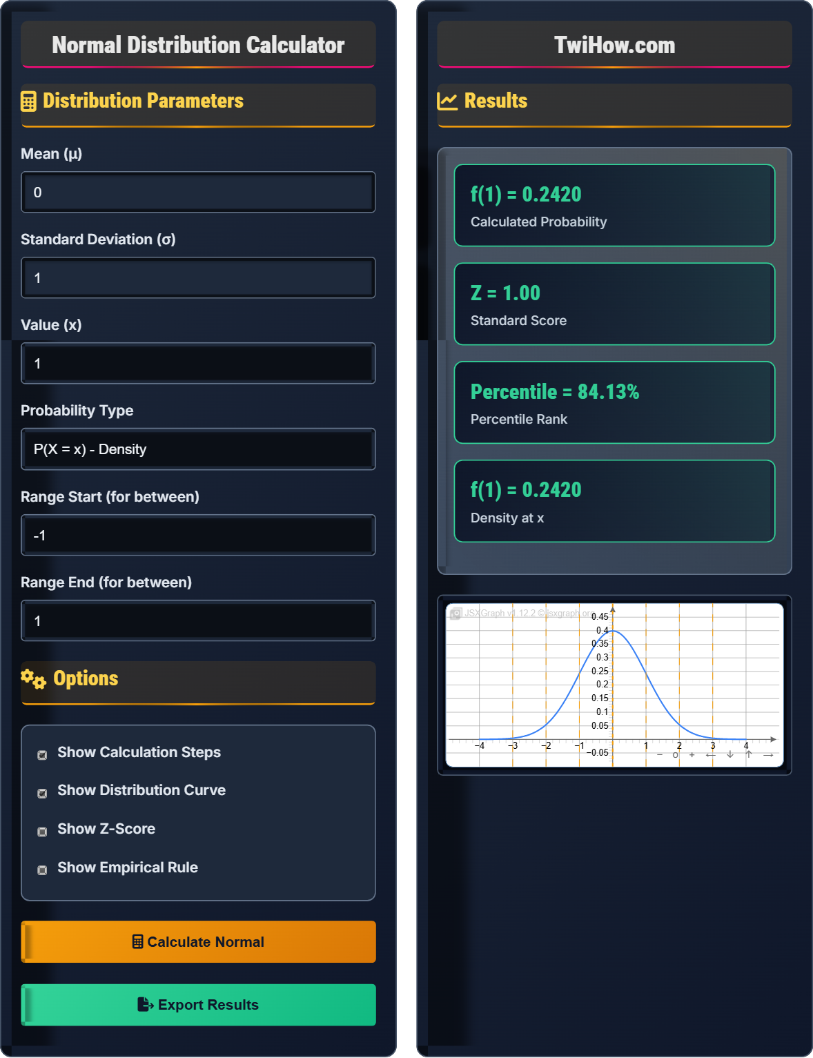
Show the calculator /Simulator\( f(x) = \frac{1}{\sigma\sqrt{2\pi}} e^{-\frac{1}{2}\left(\frac{x-\mu}{\sigma}\right)^2} \)
The normal distribution (also known as Gaussian distribution) is a continuous probability distribution characterized by its bell-shaped curve. It's symmetric around the mean (μ) and its spread is determined by the standard deviation (σ). The normal distribution is fundamental in statistics due to the Central Limit Theorem, which states that the sum of many independent random variables tends toward a normal distribution.
Where:
- \(f(x)\) = probability density at x
- \(\mu\) = mean of the distribution
- \(\sigma\) = standard deviation of the distribution
- \(e\) = Euler's number (~2.718)
- \(\pi\) = pi (~3.14159)
The normal distribution has special properties: 68% of values lie within 1σ of the mean, 95% within 2σ, and 99.7% within 3σ. This is known as the empirical rule or 68-95-99.7 rule.
Distribution Parameters
Options
Results
| x Value | Density f(x) | Cumulative P(X≤x) | Z-Score |
|---|
Enter parameters to see calculation steps.
Additional statistics will appear here.
Normal Distribution Explained
The normal distribution, also known as the Gaussian distribution or bell curve, is the most important continuous probability distribution in statistics. It describes how data values are distributed around a central value (mean) with most values clustering near the mean and fewer values as you move away from the center. The distribution is perfectly symmetric and follows a specific mathematical formula that produces its characteristic bell shape.
The probability density function of the normal distribution is:
The standard normal distribution (Z-distribution) has mean 0 and standard deviation 1:
Where:
- \(f(x)\) = probability density at point x
- \(\mu\) = population mean
- \(\sigma\) = population standard deviation
- \(X\) = raw score
- \(Z\) = standardized score (z-score)
Key characteristics of the normal distribution:
- Symmetric: Perfectly symmetric around the mean
- Bell-shaped: Highest density at the mean, decreasing towards tails
- Mean = Median = Mode: All three measures of central tendency are equal
- Empirical Rule: 68-95-99.7% of data within 1-2-3 standard deviations
- Natural Phenomena: Heights, weights, test scores
- Sampling Distributions: Means of large samples
- Measurement Errors: Random errors in experiments
- Quality Control: Manufacturing tolerances
Normal Distribution Fundamentals
The normal distribution is a continuous probability distribution that is symmetric and bell-shaped, characterized by its mean and standard deviation.
\( f(x) = \frac{1}{\sigma\sqrt{2\pi}} e^{-\frac{1}{2}\left(\frac{x-\mu}{\sigma}\right)^2} \)
Where x = value, μ = mean, σ = standard deviation.
- Completely defined by mean and standard deviation
- Area under curve = 1 (total probability)
- Symmetric about the mean
- Extends infinitely in both directions
Applications
Foundation for hypothesis testing, confidence intervals, and regression analysis.
- IQ scores and psychological testing
- Height and weight distributions
- Stock market returns
- Quality control in manufacturing
- Many real-world distributions are not perfectly normal
- Assumes infinite range of values
- Central limit theorem justifies normality
- Robust to minor departures from normality
Normal Distribution Learning Quiz
What is the probability that a standard normal random variable Z is less than 1.5? (P(Z < 1.5))
For a standard normal distribution (μ = 0, σ = 1), we need to find P(Z < 1.5).
Using the standard normal table or the empirical rule as a guide:
We know that P(Z < 1) ≈ 0.8413 and P(Z < 2) ≈ 0.9772
Since 1.5 is halfway between 1 and 2, the probability should be approximately 0.9332.
More precisely, P(Z < 1.5) = 0.9332 (from standard normal tables).
The answer is B) 0.9332.
The standard normal distribution has mean 0 and standard deviation 1. Because of its importance in statistics, probabilities for standard normal variables are tabulated in standard normal tables. The value 1.5 represents 1.5 standard deviations above the mean. Since the distribution is symmetric and most values fall within 2 standard deviations of the mean, P(Z < 1.5) should be close to 1 but less than 0.977 (the probability for 2 standard deviations).
Standard Normal Distribution: Normal distribution with μ=0 and σ=1
Z-Score: Standardized value indicating standard deviations from mean
Standard Normal Table: Lookup table for standard normal probabilities
• Standard normal has μ=0, σ=1
• P(Z < 0) = 0.5 (symmetry)
• P(Z > z) = 1 - P(Z < z)
• Remember the empirical rule (68-95-99.7)
• Use symmetry: P(Z < -z) = P(Z > z)
• Z-scores greater than 3 are rare events
• Confusing P(Z < z) with P(Z > z)
• Forgetting to standardize non-standard normal distributions
• Misreading standard normal tables
Suppose exam scores are normally distributed with mean μ = 75 and standard deviation σ = 10. What is the probability that a randomly selected student scores between 65 and 85? Also, what score corresponds to the 90th percentile?
Step 1: Calculate P(65 < X < 85)
First, convert to z-scores:
For x = 65: z₁ = (65 - 75) / 10 = -1
For x = 85: z₂ = (85 - 75) / 10 = 1
So we need P(-1 < Z < 1) = P(Z < 1) - P(Z < -1)
From standard normal table: P(Z < 1) = 0.8413 and P(Z < -1) = 0.1587
Therefore: P(65 < X < 85) = 0.8413 - 0.1587 = 0.6826 (about 68.26%)
Step 2: Find 90th percentile
We need the value x such that P(X ≤ x) = 0.90
From standard normal table, P(Z ≤ 1.28) ≈ 0.90
Using the inverse transformation: x = μ + zσ = 75 + 1.28(10) = 75 + 12.8 = 87.8
The probability of scoring between 65 and 85 is 68.26%, and the 90th percentile score is 87.8.
This problem demonstrates two important applications of the normal distribution: calculating probabilities and finding percentiles. To calculate probabilities for any normal distribution, we standardize by converting to z-scores using the formula Z = (X - μ) / σ. This allows us to use the standard normal table. For percentile problems, we first find the z-score corresponding to the desired probability and then convert back to the original scale.
Percentile: Value below which a percentage of observations fall
Z-Score: Number of standard deviations from the mean
Standardization: Converting to standard normal scale
• Z = (X - μ) / σ for standardization
• X = μ + Zσ for reverse transformation
• Percentiles correspond to cumulative probabilities
• Always sketch the distribution first
• Standardize before using normal tables
• Check that your answer makes sense
• Forgetting to standardize before using normal tables
• Confusing z-scores with raw scores
• Not checking if the answer is reasonable
The diameter of ball bearings produced by a factory follows a normal distribution with mean 10mm and standard deviation 0.2mm. The specification limits are 9.6mm to 10.4mm. What percentage of ball bearings will be rejected for not meeting specifications?
Step 1: Identify the problem
We need to find P(X < 9.6 or X > 10.4) = P(X < 9.6) + P(X > 10.4)
Step 2: Standardize the limits
For x = 9.6: z₁ = (9.6 - 10) / 0.2 = -2
For x = 10.4: z₂ = (10.4 - 10) / 0.2 = 2
Step 3: Calculate probabilities
P(X < 9.6) = P(Z < -2) = 0.0228
P(X > 10.4) = P(Z > 2) = 1 - P(Z < 2) = 1 - 0.9772 = 0.0228
Step 4: Calculate total rejection rate
Rejection rate = 0.0228 + 0.0228 = 0.0456 = 4.56%
About 4.56% of ball bearings will be rejected for not meeting specifications.
This quality control problem shows how the normal distribution is used in manufacturing. The empirical rule tells us that about 95% of values fall within 2 standard deviations of the mean. Since our specification limits are exactly 2 standard deviations from the mean (10 ± 2×0.2), we expect about 5% to be outside the limits. The normal distribution provides the precise calculation for this percentage.
Specification Limits: Acceptable range for product characteristics
Rejection Rate: Percentage of defective products
Quality Control: Process of ensuring product meets specifications
• P(outside limits) = P(below lower) + P(above upper)
• Specification limits define acceptable range
• Normal distribution models many physical measurements
• Use symmetry when limits are equidistant from mean
• Consider process capability indices
• Monitor both mean and standard deviation
• Only calculating one tail (below or above)
• Forgetting to standardize both limits
• Not considering that both tails contribute to rejects
The average height of adult males in a population is 70 inches with a standard deviation of 3 inches. If we randomly select a sample of 36 men, what is the probability that the sample mean height is between 69.5 and 70.5 inches?
Step 1: Apply Central Limit Theorem
For sample means, the sampling distribution is normal with:
Mean of sample means: μₓ̄ = μ = 70 inches
Standard deviation of sample means: σₓ̄ = σ/√n = 3/√36 = 3/6 = 0.5 inches
Step 2: Standardize the sample mean values
For x̄ = 69.5: z₁ = (69.5 - 70) / 0.5 = -1
For x̄ = 70.5: z₂ = (70.5 - 70) / 0.5 = 1
Step 3: Calculate probability
P(69.5 < X̄ < 70.5) = P(-1 < Z < 1) = P(Z < 1) - P(Z < -1)
= 0.8413 - 0.1587 = 0.6826
The probability that the sample mean height is between 69.5 and 70.5 inches is approximately 68.26%.
The Central Limit Theorem states that the sampling distribution of the sample mean approaches a normal distribution as the sample size increases, regardless of the population distribution. The key insight is that the standard deviation of the sample means (called the standard error) is σ/√n, which is smaller than the population standard deviation. This means sample means cluster more tightly around the population mean than individual observations.
Central Limit Theorem: Sample means approach normal distribution
Standard Error: Standard deviation of sampling distribution
Sampling Distribution: Distribution of sample statistics
• Sample mean distribution: μₓ̄ = μ
• Sample mean standard deviation: σₓ̄ = σ/√n
• CLT applies for n ≥ 30 (usually)
• Always identify if dealing with sample means
• Use standard error (σ/√n) for sample means
• Sample means have less variability than individual values
• Using population standard deviation instead of standard error
• Forgetting to divide by √n
• Not recognizing when CLT applies
Which of the following statements about the normal distribution is TRUE?
Let's examine each option:
A) False - In a normal distribution, the mean, median, and mode are all equal due to perfect symmetry
B) False - The normal distribution is perfectly symmetric, not skewed
C) True - Due to the symmetric, bell-shaped nature of the normal distribution, the mean, median, and mode all coincide at the center
D) False - The normal distribution has light tails (exponentially decreasing), not heavy tails
The normal distribution is perfectly symmetric about its mean, which means the mean (average), median (middle value), and mode (most frequent value) all occur at the same point - the center of the distribution.
The answer is C) The mean, median, and mode are all equal.
This is a fundamental property of the normal distribution that stems from its perfect symmetry. In any symmetric distribution, the mean, median, and mode are equal. However, in skewed distributions, these measures differ. The normal distribution's symmetry ensures that 50% of the data lies below the mean and 50% lies above, making the median equal to the mean. The mode equals the mean because the distribution peaks at the center.
Mean: Average value of the distribution
Median: Middle value when data is ordered
Mode: Most frequently occurring value
• Mean = Median = Mode in normal distribution
• Perfect symmetry around mean
• Light tails (exponential decay)
• Remember the symmetry property
• Use empirical rule for quick estimates
• Check if distribution is approximately symmetric
• Confusing with skewed distributions
• Thinking normal distribution has heavy tails
• Not recognizing symmetry property
FAQ
Q: What is the difference between the normal distribution and the standard normal distribution?
A: The normal distribution is a family of distributions that can have any mean (μ) and any positive standard deviation (σ). The standard normal distribution is a specific member of this family with mean μ = 0 and standard deviation σ = 1. Any normal distribution can be converted to a standard normal distribution using the z-score transformation: Z = (X - μ) / σ. This standardization allows us to use standard normal tables to find probabilities for any normal distribution.
Q: Why is the normal distribution so important in statistics?
A: The normal distribution is fundamental due to the Central Limit Theorem, which states that the sum (or average) of many independent random variables approaches a normal distribution regardless of the original distribution. This makes it applicable to sample means, proportions, and many real-world phenomena. Additionally, many statistical methods assume normality, and the distribution has nice mathematical properties that make calculations tractable. It also provides a good approximation for many natural and social phenomena.