Best Practices for Inventory Optimization and Demand Forecasting
Supply chain management guide • Step-by-step explanations
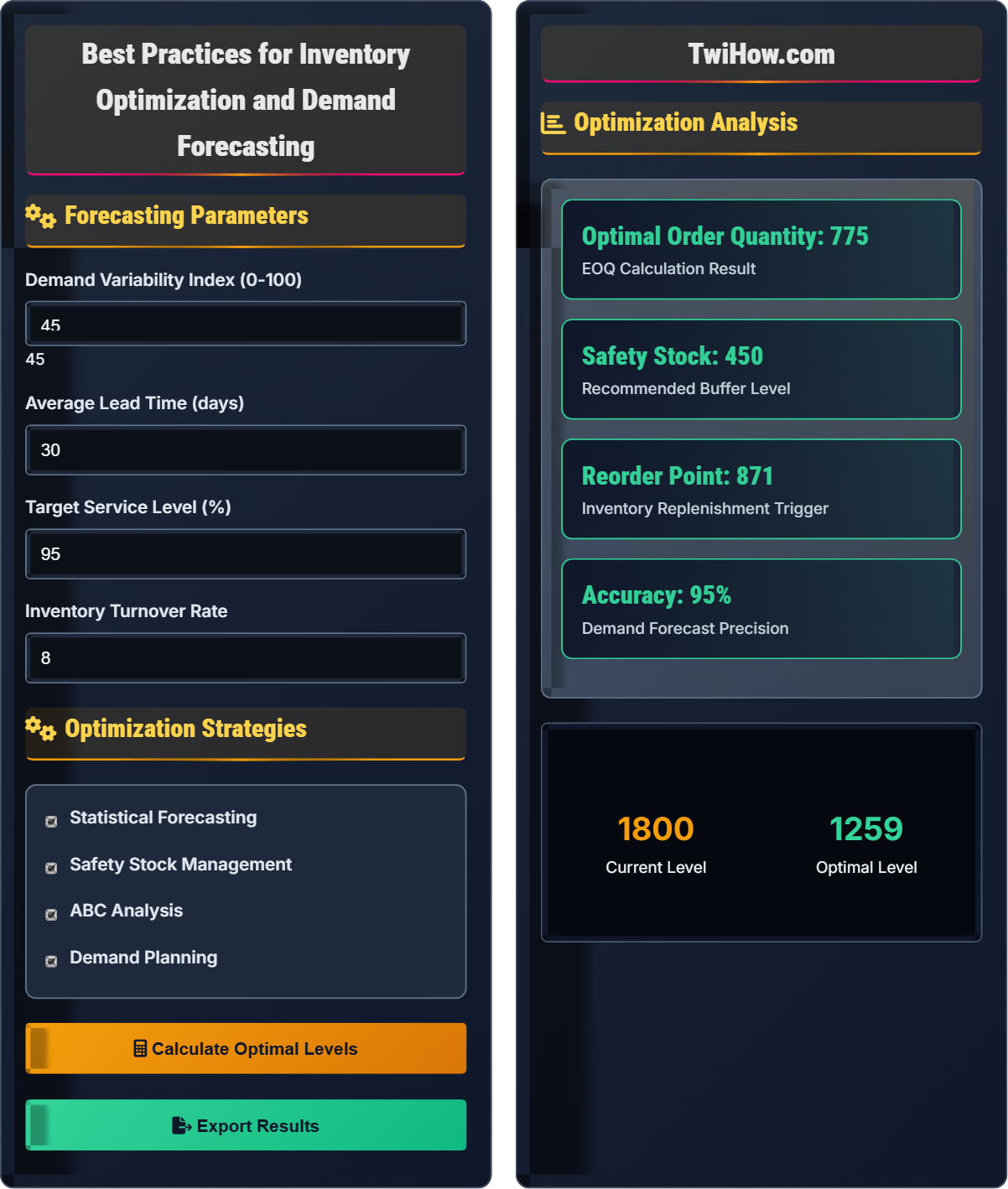
Inventory & Forecasting:
Show Forecasting CalculatorInventory optimization and demand forecasting are critical components of effective supply chain management. These practices involve using data analytics, statistical methods, and market intelligence to predict customer demand accurately and maintain optimal inventory levels. By implementing best practices, companies can reduce carrying costs, minimize stockouts, improve customer satisfaction, and enhance overall operational efficiency.
Key best practices include:
- Historical Analysis: Using past demand patterns to predict future needs
- Safety Stock Management: Maintaining buffers for uncertainty
- ABC Classification: Prioritizing inventory based on value and importance
- Seasonal Adjustments: Accounting for predictable demand fluctuations
- Technology Integration: Using advanced analytics and AI for forecasting
Successful inventory and forecasting practices balance cost efficiency with service level requirements, ensuring optimal performance across the entire supply chain.
Forecasting Parameters
Optimization Strategies
Optimization Analysis
| Parameter | Current | Optimal | Improvement |
|---|---|---|---|
| Inventory Level | 1,800 | 1,700 | 5.6% reduction |
| Service Level | 90% | 95% | 5% improvement |
| Turnover Rate | 7.2 | 8.0 | 11% improvement |
| Carrying Cost | $18,000 | $17,000 | $1,000 savings |
| Stockout Risk | 8% | 5% | 3% reduction |
Recommended Actions
- Implement statistical forecasting models
- Optimize safety stock levels based on demand variability
- Apply ABC analysis for inventory prioritization
- Establish regular demand planning cycles
- Monitor forecast accuracy and adjust models
Implementation Benefits
- Reduced carrying costs
- Improved service levels
- Lower stockout risk
- Better cash flow management
- Enhanced customer satisfaction
Inventory Optimization and Demand Forecasting Best Practices
Inventory optimization is the process of determining the optimal level of inventory to maintain across the supply chain to satisfy demand while minimizing costs. It involves balancing carrying costs, stockout costs, and ordering costs to achieve the most efficient inventory management. The goal is to have the right products in the right quantities at the right locations and times.
The Economic Order Quantity (EOQ) formula:
Where:
- D: Annual demand (units)
- S: Ordering cost per order
- H: Holding cost per unit per year
Reorder Point (ROP) formula:
Key demand forecasting approaches:
- Statistical Methods: Moving averages, exponential smoothing, regression analysis
- Qualitative Methods: Expert opinions, market research, Delphi method
- Collaborative Planning: Joint forecasting with suppliers and customers
- Advanced Analytics: Machine learning, AI-based forecasting
- Seasonal Adjustments: Accounting for predictable demand patterns
- Trend Analysis: Identifying long-term demand movements
- Walmart: Uses advanced analytics for demand forecasting and inventory optimization
- Zara: Implements fast fashion model with optimized inventory cycles
- Toyota: Just-in-time inventory system with precise forecasting
- Amazon: Predictive analytics for inventory placement and demand planning
- Procter & Gamble: Collaborative planning with retailers for demand forecasting
Core Concepts
EOQ, safety stock, reorder point, demand forecasting, inventory turnover, carrying costs, stockout costs, ABC analysis, service level, lead time.
Optimal Inventory = (Demand Forecast × Lead Time) + Safety Stock + Seasonal Adjustments
Where safety stock = Z-score × Standard Deviation of Demand × √Lead Time
- Balance cost and service level
- Use data-driven approaches
- Regularly update forecasts
- Segment inventory strategically
Implementation Strategies
Statistical forecasting, safety stock management, ABC analysis, demand planning, seasonal adjustments, collaborative forecasting.
- Collect and analyze historical demand data
- Select appropriate forecasting methods
- Calculate safety stock levels
- Determine optimal order quantities
- Implement inventory management systems
- Monitor and refine processes
- Update forecasts regularly
- Use multiple forecasting methods
- Consider seasonality and trends
- Maintain accurate data
Inventory & Forecasting Quiz
What does the Economic Order Quantity (EOQ) formula primarily balance?
The EOQ formula balances carrying costs (costs of holding inventory) with ordering costs (costs of placing orders). The optimal order quantity minimizes the total of these two costs. As order size increases, carrying costs increase while ordering costs decrease, and vice versa.
The answer is B) Carrying costs and ordering costs.
The EOQ model demonstrates a fundamental trade-off in inventory management. Larger order quantities reduce the frequency of orders (lowering ordering costs) but increase average inventory levels (raising carrying costs). Smaller orders reduce carrying costs but increase ordering costs. The EOQ finds the sweet spot where total costs are minimized.
EOQ: Economic Order Quantity - optimal order size
Carrying Costs: Costs of holding inventory (storage, insurance, etc.)
Ordering Costs: Costs of placing orders (processing, shipping, etc.)
• EOQ assumes constant demand
• Balances two opposing cost factors
• Assumes instantaneous replenishment
• Use historical data for accurate inputs
• Consider quantity discounts in calculations
• Update EOQ regularly as costs change
• Using outdated cost data
• Not considering quantity discounts
• Ignoring demand variability
Explain how to calculate safety stock and why it's important for inventory optimization. What factors influence the amount of safety stock needed?
Safety Stock Formula:
Safety Stock = Z-score × Standard Deviation of Demand × √Lead Time
Importance: Safety stock acts as a buffer against demand and supply uncertainties, preventing stockouts while maintaining desired service levels.
Factors Influencing Safety Stock:
1. Demand Variability: Higher variation requires more safety stock
2. Lead Time Variability: Unpredictable lead times need more buffer
3. Service Level: Higher service targets require more safety stock
4. Lead Time Length: Longer lead times increase safety stock needs
5. Cost Considerations: Balance stockout costs vs. carrying costs
Safety stock represents a fundamental trade-off in inventory management. Too little safety stock increases stockout risk, leading to lost sales and customer dissatisfaction. Too much safety stock increases carrying costs and ties up capital. The calculation considers both demand uncertainty and supply uncertainty, using statistical methods to determine appropriate buffer levels.
Safety Stock: Extra inventory to protect against uncertainties
Z-score: Statistical measure of confidence level
Standard Deviation: Measure of demand variability
• Safety stock should be based on statistical analysis
• Regularly review and adjust safety stock levels
• Consider both demand and supply variability
• Use historical data to estimate variability
• Segment safety stock by product importance
• Consider supplier reliability in calculations
• Using arbitrary safety stock levels
• Not considering seasonal variations
• Failing to update calculations regularly
A company has annual demand of 10,000 units, ordering cost of $50 per order, and carrying cost of $2 per unit per year. Calculate the Economic Order Quantity (EOQ) and determine how many orders should be placed annually.
EOQ Formula: EOQ = √(2DS/H)
Where:
D = Annual demand = 10,000 units
S = Ordering cost = $50 per order
H = Carrying cost = $2 per unit per year
Calculation:
EOQ = √(2 × 10,000 × 50 / 2)
EOQ = √(1,000,000 / 2)
EOQ = √500,000
EOQ = 707.1 ≈ 707 units
Number of Orders: 10,000 / 707 = 14.1 ≈ 14 orders per year
This calculation demonstrates the practical application of the EOQ formula. The company should order approximately 707 units each time to minimize total inventory costs. This results in about 14 orders per year. The EOQ model helps balance the trade-off between carrying costs (which favor smaller, more frequent orders) and ordering costs (which favor larger, less frequent orders).
EOQ: Economic Order Quantity - optimal order size
Annual Orders: Total demand divided by order quantity
Cost Optimization: Minimizing total inventory costs
• EOQ assumes constant demand and costs
• Round to practical order quantities
• Verify assumptions are valid
• Consider quantity discounts when applicable
• Round to convenient batch sizes
• Update calculations as costs change
• Using incorrect units in calculations
• Not considering quantity discounts
• Failing to update as conditions change
A retail company has the following products with their annual value contributions: Product A ($50,000), Product B ($30,000), Product C ($15,000), Product D ($10,000), Product E ($5,000). Perform an ABC analysis and explain how this should influence inventory management strategies for each product category.
ABC Analysis:
Total Annual Value: $50,000 + $30,000 + $15,000 + $10,000 + $5,000 = $110,000
Product A: $50,000 / $110,000 = 45.5% → Category A
Product B: $30,000 / $110,000 = 27.3% → Category A (Cumulative: 72.8%)
Product C: $15,000 / $110,000 = 13.6% → Category B (Cumulative: 86.4%)
Product D: $10,000 / $110,000 = 9.1% → Category C (Cumulative: 95.5%)
Product E: $5,000 / $110,000 = 4.5% → Category C (Cumulative: 100%)
Management Strategies: A-items: Tight control, frequent monitoring, accurate forecasting. B-items: Moderate control. C-items: Simple control, periodic review.
ABC analysis follows the Pareto principle (80/20 rule), where a small percentage of items account for a large percentage of value. This analysis helps prioritize management effort and resources. Category A items require the most attention and sophisticated management techniques since they represent the majority of inventory value. Category C items can be managed with simpler, less intensive methods.
ABC Analysis: Classification based on annual consumption value
Category A: High-value items (typically 70-80% of value)
Category B: Medium-value items (typically 15-20% of value)
• Focus management efforts on high-value items
• Use appropriate control methods by category
• Review classifications periodically
• Consider other factors besides value (criticality, demand variability)
• Use ABC analysis for multiple criteria
• Update classifications regularly
• Only considering monetary value
• Not updating classifications regularly
• Applying same controls to all categories
Which metric is most commonly used to measure forecast accuracy?
All of these metrics are commonly used to measure forecast accuracy. MAPE is particularly popular because it expresses error as a percentage, making it easy to interpret. MAD measures average error magnitude, and RMSE penalizes larger errors more heavily. Each metric has its advantages depending on the specific use case.
The answer is D) All of the above.
Forecast accuracy measurement is crucial for continuous improvement. MAPE is widely used because it's scale-independent and easy to understand. MAD provides straightforward interpretation of average error. RMSE is sensitive to outliers, which can be important when large errors are particularly costly. The choice of metric depends on business priorities and the cost structure of forecast errors.
MAPE: Mean Absolute Percentage Error - average percentage error
MAD: Mean Absolute Deviation - average absolute error
RMSE: Root Mean Square Error - considers squared errors
• Use multiple metrics for comprehensive evaluation
• Consider business impact of different error types
• Track accuracy over time
• Use MAPE for reporting to management
• Consider weighted metrics for different products
• Track accuracy by product category
• Using only one metric for evaluation
• Not considering business impact of errors
• Failing to track accuracy trends
FAQ
Q: How often should we update our demand forecasts?
A: Forecast update frequency depends on your business characteristics:
1. Fast-moving products: Weekly or daily updates
2. Slow-moving products: Monthly or quarterly updates
3. Seasonal products: More frequent updates during peak seasons
4. Stable products: Monthly updates with quarterly reviews
Generally, update forecasts monthly with weekly exception reporting. The key is balancing accuracy improvement with administrative costs.
Q: What's the difference between demand planning and forecasting?
A: Forecasting is a component of demand planning:
Forecasting: Statistical process of predicting future demand based on historical data and trends
Demand Planning: Broader process that includes forecasting plus business inputs, collaboration, and consensus building
Demand planning incorporates:
• Statistical forecasts
• Business intelligence (promotions, new products)
• Customer input and market intelligence
• Cross-functional collaboration
• Final consensus forecast
Demand planning is the strategic process; forecasting is the tactical tool.